Lab 5

Lab 5

Introduction:

The purpose of the previous lab was to  to construct a elevation surface model of terrain that our group constructed in a square meter "sandbox". We wanted to make sure we measured the entire box to make sure we captured all of the elevation change. We used stratified sampling by measuring out even plots for the entire "sandbox". All of the plots we of equal size. In order to read the data in a GIS we needed to normalize the data. Data normalization is the process of organizing the data at hand in a certain way to retain and improve data integrity. It was important that the data in the excel spreadsheet was normalized so that way there would be zero problems in the future with the data. The data points did not have a coordinate system, so they were displayed in the same box like representation of the sandbox. Since we had 3 coordinates (X, Y, and Z), we could map the elevation since we had the 'latitude and longitude'.


Methods:

Since the sandbox project was a large production, the creation of a geodatabase was inevitable. Once each person had their own geodatabase in their own folder, we could start importing our data. We took the excel spreadsheet we had stored our data points and imported it into the geodatabase. This was able to happen in a smooth manner because the data was set to 'numeric' and had the proper decimal values. Once the data was normalized, I used the add 'XY data' function to bring the data into ArcMap. Figure 1 below is what the data points looked like once they were converted into a point feature class.

Figure 1: The data points in a GIS

Once the point feature class was set up, it was time to experiment with different interpolation methods, and different parameters within those methods. There were 5 different methods that were a realistic representation of the terrain. The 5 methods are the following: IDW (inverse distance weighted), Natural Neighbors, Kriging, Spline, and TIN. The IDW method assumes that things that are close to one another are more alike than those that are farther apart. It is effective with the calculations, but it does not create an exact model of the data. The Natural Neighbor method is used often because of it provides a smoother approximation to the underlying whole of the data. This is a great method to use when looking for a smooth representation of the data. The Kriging method effectively involves an interactive investigation of the spatial behavior of the phenomenon represented by the z-values before you select the best estimation method for generating the output surface. A large scale model would look better using this method than a small scale model. The spline test uses a special type of piece wise polynomial called a spline. This type of modeling is popular because of the smooth end result. The TIN comprises a triangular network of vertices with associated coordinated in three dimensions. The end result is not a smooth model, but rather an array of polygons connected to create the terrain based off of the data points.

Results/Discussion:

The IDW method assumes that things that are close to one another are more alike than those that are farther apart. Figure 2 below is what the IDW model looks like with my data points. A major downside of this method is that each point is effected by the calculations. The map almost looks bubbly with all of the points making an impact on the terrain.

Figure 2: IDW interpolation method

Figure 3 below is the Natural Neighbor interpolation model. This model looks almost exactly like the model my group built in the sand. The color scheme helps a lot because the low places are in blue and the high places in red. The Natural Neighbor method is used often because of it provides a smoother approximation to the underlying whole of the data. This is my favorite method to represent this set of data. If you're looking for an interpolation method that shows rough terrain, the Natural Neighbor method is not the one for you.

Figure 3: Natural Neighbor interpolation method

Figure 4 below was created using the Kriging interpolation method. The features on the surface model are not as prevalent as the other models created. This is not a very good representation of what was built in the sand. The Kriging method effectively involves an interactive investigation of the spatial behavior of the phenomenon represented by the z-values before you select the best estimation method for generating the output surface. Like other interpolation methods, the Kriging method generates an estimated surface from a scattered set of points with z-values. This would be a good interpolation method for a large study area with a large elevation changes.
 

Figure 4: Kriging interpolation method

The spline test is demonstrated in figure 5 below. The spline test for my particular data is a very close representation of my data points. The spline test uses a special type of piece wise polynomial called a spline. Figure 5 shows a nice representation of what the terrain looked like in the sandbox. I am also a fan of using this method to show the data points. It gives a smooth representation of the data. Spline interpolation avoids the problem that can occur between points when interpolating using high degree polynomials. 

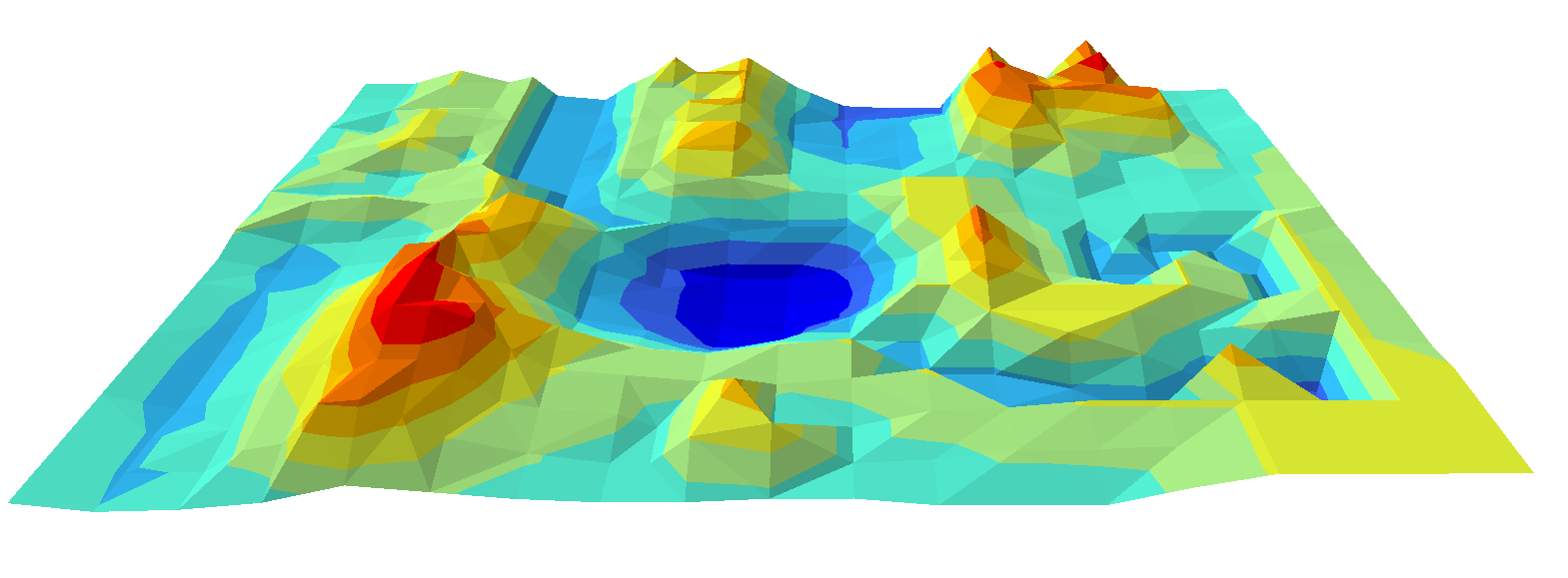
Figure 5: Spline interpolation method

Figure 6 is an example of the TIN interpolation method. This method shows the elevation very nicely in the image below. A triangulated irregular network, TIN, comprises a triangular network of vertices with associated coordinated in three dimensions. This method is useful if there are three dimensions to map. If you're looking for a smooth model, this method is not the one for you. Figure 6 is also one of my favorite representations of the data points. 

Figure 6: TIN interpolation method

For the purpose of this lab, the IDW method is not suitable. In the future, I would like to see a more extreme landscape with each interpolation method. The northeastern corner of the map was supposed to be a volcano, but it just came out a large uneven mountain. This is something that can be improved upon. One area I would like to point out is the '5' in the middle right of the images. It is most obvious on the TIN model, but since we were group 5, we figured we would try and create a '5' in the landscape.

Conclusion:

This survey relates to all field based surveys that involve retrieving the elevation coordinate. If the data in the field based survey has three coordinates, a interpolation model can be achieved. The interpolation methods can be used for other things aside from elevation. One possible use might be for precipitation. As long as a third coordinate with meaning is included in the data, an interpolation model can be created. Each field excursion is different, so there are some minor things that would/will change for each method, but the process of creating the model will remain the same. The scales and projections will change and the elevation change will also change for terrains in other surveys. It is absolutely not realistic to create the detailed grid survey as we did in this lab. The materials may be limited in the field as well as the study area may be to large to create a grid system the way we did in lab. The smaller the grid system the more likely the data will be more accurate. It is unrealistic to lay a grid system on any plot of land that is not 100% controlled.


Sources:
ArcGISHelp