Lab 6

Lab 6

Introduction:

The purpose of this lab is to conduct a survey with a grid based coordinate system. The techniques learned in this lab are to be used when 'technology' is not readily available or usable. It is important to be able to follow through with a survey no matter the measurement tools at hand. For this lab, we are to preform a survey in Putnam Park. The survey is to be conducted by using distance and azimuth. This method is a very basic survey technique, and is similar to the point-quarter method and mapping out linear features on the landscape. The distance and azimuth method uses a handheld compass and a handheld rangefinder. While out in the field, we also learned about the following survey equipment: a GPS, tape reel, and a sonic distance finder.

Study Area:

The study area for this lab is Putnam Park Drive. We were on the gravel path with our backs to the ridge looking out into the swampy marsh area. We recorded the coordinates for one place and took each measurement from that exact spot. The coordinates for each point of origin (there were three points for the entire class) were recorded and shared throughout the class. Each point of origin had the distance and azimuth for ten different trees in Putnam Park. 

Methods:

After choosing the point where we were going to take our points from, we needed to retrieve the coordinates of the point of origin. The Bad Elf GPS gave us the coordinate point and we recorded it in our field notebooks. All of the groups used this GPS to attain their point of origin. We then proceeded to record the distances of the trees to the point of origin with the laser targeting range finder II. We then recorded the azimuth with the Suunto compass. The compass was previously adjusted 1 degree for declination. Figure 1 below shows two of my colleagues using both of the measuring tools we used to gather our information.

Figure 1: Colleague 1 on the left using the Laser to find the distance,
and colleague 2 on the right using the compass to find the azimuth 

 The laser gave the distance in meters of how far the tree was from the point of origin. The compass gave the azimuth of the tree in regarding its angle to the point of origin. We also recorded two other attributes along with distance and azimuth. We recorded the diameter of the tree as well as the type of tree. Figure 2 below shows another one of my colleagues reading the tape reel and recording the diameter of the tree in centimeters.

Figure 2: Colleague 3 using the tape reel to measure the diameter of the tree trunk

Once all of the data were recorded, we entered the data into a spreadsheet everyone could access. From there I took the data and normalized it. Once the data was normalized it looked like figure 3 below. 

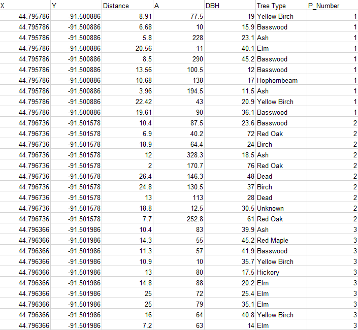
Figure 3: The normalized data from the tree survey

The table above is the final excel file before it was imported into a GIS. The goal of using the GIS is to create a digital survey map. In order to do this, we had to use the 'Bearing Distance to Line' tool in ArcGIS. The tool created lines extending from the point of origin. This is an extremely helpful tool to visually show the distances of points from the point of origin. Figure 4 below shows the lines representing the distance from the point of origin to the tree. 

Figure 4: The 'Bearing Distance' tool created the lines from the point of origin

The bearing distance tool is helpful in showing the distance of the trees to the point of origin. Figure 5 below represents the vertices of each tree point.

Figure 5: The 'Features Vertices to Points' tool creates points at the end of each distance line

In order to create the points, the tool 'Features Vertices to Points' had to be used. The tool is located under the data management tools in the toolbox in ArcMap. It essentially creates a point where each tree, or whatever is being recorded, is located. The tool just creates a point at each vertex of every distance line.

Results/Discussion:

After creating a digital image in a GIS, the distances and azimuths for each tree seemed to differ greatly. I would not suggest this method of retrieving data to anyone who wants an accurate data set. The readings of the distance finder and azimuth had some large differences, and this is because of human error. All six group members took each type of measurement and that in and of itself results in error. There is also the fact that we are different heights and we were not standing on the exact point of origin 100% of the time. After we recorded out point of origins coordinates, we went to use the sonic distance finder to survey the trees. The sonic distance finder did not work for my group, so we had to revert to using the laser targeting range finder II. Technological difficulties occur even when the survey equipment seems unbreakable. This particular solution was solved by using a different distance measuring tool, the laser targeting range finder II. All of these tools are accurate enough to retrieve points and data that is close to the actual numeric value. 

Conclusions:

If you know the exact point of origin down to the coordinates, it is possible to use the distance azimuth surveying method to attain data even though a GPS is not at hand. The better the equipment, the more accurate the data results will be. If this survey was to be recreated, I would go with the point quarter survey. The point quarter survey takes random survey points in a measured out grid with four large quadrants. I believe it is crucial to know how to use the distance azimuth survey method for future endeavors when the use of technology is not permitted or accessible. 

Lab 5

Lab 5

Introduction:

The purpose of the previous lab was to  to construct a elevation surface model of terrain that our group constructed in a square meter "sandbox". We wanted to make sure we measured the entire box to make sure we captured all of the elevation change. We used stratified sampling by measuring out even plots for the entire "sandbox". All of the plots we of equal size. In order to read the data in a GIS we needed to normalize the data. Data normalization is the process of organizing the data at hand in a certain way to retain and improve data integrity. It was important that the data in the excel spreadsheet was normalized so that way there would be zero problems in the future with the data. The data points did not have a coordinate system, so they were displayed in the same box like representation of the sandbox. Since we had 3 coordinates (X, Y, and Z), we could map the elevation since we had the 'latitude and longitude'.


Methods:

Since the sandbox project was a large production, the creation of a geodatabase was inevitable. Once each person had their own geodatabase in their own folder, we could start importing our data. We took the excel spreadsheet we had stored our data points and imported it into the geodatabase. This was able to happen in a smooth manner because the data was set to 'numeric' and had the proper decimal values. Once the data was normalized, I used the add 'XY data' function to bring the data into ArcMap. Figure 1 below is what the data points looked like once they were converted into a point feature class.

Figure 1: The data points in a GIS

Once the point feature class was set up, it was time to experiment with different interpolation methods, and different parameters within those methods. There were 5 different methods that were a realistic representation of the terrain. The 5 methods are the following: IDW (inverse distance weighted), Natural Neighbors, Kriging, Spline, and TIN. The IDW method assumes that things that are close to one another are more alike than those that are farther apart. It is effective with the calculations, but it does not create an exact model of the data. The Natural Neighbor method is used often because of it provides a smoother approximation to the underlying whole of the data. This is a great method to use when looking for a smooth representation of the data. The Kriging method effectively involves an interactive investigation of the spatial behavior of the phenomenon represented by the z-values before you select the best estimation method for generating the output surface. A large scale model would look better using this method than a small scale model. The spline test uses a special type of piece wise polynomial called a spline. This type of modeling is popular because of the smooth end result. The TIN comprises a triangular network of vertices with associated coordinated in three dimensions. The end result is not a smooth model, but rather an array of polygons connected to create the terrain based off of the data points.

Results/Discussion:

The IDW method assumes that things that are close to one another are more alike than those that are farther apart. Figure 2 below is what the IDW model looks like with my data points. A major downside of this method is that each point is effected by the calculations. The map almost looks bubbly with all of the points making an impact on the terrain.

Figure 2: IDW interpolation method

Figure 3 below is the Natural Neighbor interpolation model. This model looks almost exactly like the model my group built in the sand. The color scheme helps a lot because the low places are in blue and the high places in red. The Natural Neighbor method is used often because of it provides a smoother approximation to the underlying whole of the data. This is my favorite method to represent this set of data. If you're looking for an interpolation method that shows rough terrain, the Natural Neighbor method is not the one for you.

Figure 3: Natural Neighbor interpolation method

Figure 4 below was created using the Kriging interpolation method. The features on the surface model are not as prevalent as the other models created. This is not a very good representation of what was built in the sand. The Kriging method effectively involves an interactive investigation of the spatial behavior of the phenomenon represented by the z-values before you select the best estimation method for generating the output surface. Like other interpolation methods, the Kriging method generates an estimated surface from a scattered set of points with z-values. This would be a good interpolation method for a large study area with a large elevation changes.
 

Figure 4: Kriging interpolation method

The spline test is demonstrated in figure 5 below. The spline test for my particular data is a very close representation of my data points. The spline test uses a special type of piece wise polynomial called a spline. Figure 5 shows a nice representation of what the terrain looked like in the sandbox. I am also a fan of using this method to show the data points. It gives a smooth representation of the data. Spline interpolation avoids the problem that can occur between points when interpolating using high degree polynomials. 

Figure 5: Spline interpolation method

Figure 6 is an example of the TIN interpolation method. This method shows the elevation very nicely in the image below. A triangulated irregular network, TIN, comprises a triangular network of vertices with associated coordinated in three dimensions. This method is useful if there are three dimensions to map. If you're looking for a smooth model, this method is not the one for you. Figure 6 is also one of my favorite representations of the data points. 

Figure 6: TIN interpolation method

For the purpose of this lab, the IDW method is not suitable. In the future, I would like to see a more extreme landscape with each interpolation method. The northeastern corner of the map was supposed to be a volcano, but it just came out a large uneven mountain. This is something that can be improved upon. One area I would like to point out is the '5' in the middle right of the images. It is most obvious on the TIN model, but since we were group 5, we figured we would try and create a '5' in the landscape.

Conclusion:

This survey relates to all field based surveys that involve retrieving the elevation coordinate. If the data in the field based survey has three coordinates, a interpolation model can be achieved. The interpolation methods can be used for other things aside from elevation. One possible use might be for precipitation. As long as a third coordinate with meaning is included in the data, an interpolation model can be created. Each field excursion is different, so there are some minor things that would/will change for each method, but the process of creating the model will remain the same. The scales and projections will change and the elevation change will also change for terrains in other surveys. It is absolutely not realistic to create the detailed grid survey as we did in this lab. The materials may be limited in the field as well as the study area may be to large to create a grid system the way we did in lab. The smaller the grid system the more likely the data will be more accurate. It is unrealistic to lay a grid system on any plot of land that is not 100% controlled.


Sources:
ArcGISHelp

Lab 4: Creating a Digital Elevation Surface Model using critical thinking skills and improvised survey techniques

Lab 4

Introduction:

The purpose of this lab is to construct a elevation surface model of terrain that our group constructed in a square meter "sandbox". In order to gather points, we needed to figure out what type of sampling we wanted to conduct. There are many different ways to sample points in any given model. The three main types of sampling are random, systematic, and stratified. Random sampling has the least amount of bias, but it could lead to a poor representation of the overall area in question. Systematic sampling samples the majority of the study area using set intervals, but is more biased and can lead to over or under representation of the area. Stratified sampling can generate accurate results that represent the study area as a whole, and it's flexible when it comes to data correlations and comparisons. The one major disadvantage of stratified sampling is that is that the proportions of the areas in question must be known and accurate. Random sampling was not a good choice, because we needed a structured sampling system. Stratified sampling was not an ideal choice either because we wanted to measure the entire box, not just small portions of the box. We wanted to make sure we measured the entire box to make sure we captured all of the elevation change. We used systematic sampling by measuring out even plots for the entire "sandbox". All of the plots we of equal size. It is important that we chose the correct sampling method because we want to know elevation changes which can occur rapidly in many areas, so choosing a sampling method that covers the entire area is critical.

Methods:

My group and myself chose the systematic sampling method. We chose this method because it seemed to make the most sense since we were working with primarily elevation. We wanted to make a grid to make sure we collected a data point from every spot on the model. We created a grid system that allowed us to record a data point ever 6 cm. Figure 1 below shows the 114 cm by 114 cm "sandbox" that was the study area for this lab.

Figure 1: The study area terrain model

As seen in figure 1, there are pushpins outlining the study area. We placed a pushpin on the perimeter of the sandbox every 6 cm. We chose 6 cm because 6 cm x 19 cm = 114 cm. This means there were 19 columns and 19 rows resulting in 361 6 cm by 6 cm plots. The string was then wrapped around the pushpins creating a grid system. Figure 2 below depicts the grid system nearly complete.

Figure 2: The grid system that was used to record data points

The study area/sandbox is located in a backyard near Philips Hall. The backyard is across the road from the Philips Hall garage/shed. In order to create our sampling system, we needed measurement tools. In order to start our lab, we had to create a terrain model with the following landforms: ridge, hill, depression, valley, and plain. We used meter sticks to measure out and place pushpins every 6 cm. We then used string to create our grid system. In order to create the elevation model, collecting the "z coordinate" was critical. We chose to have the top of the wood of the sandbox be sea-level. This meant everything below the wooden sandbox was below sea-level, and the data points that were above the wood were above sea-level. In some areas where elevation relief was steep, we took two points which, in a sense, split the plot in half. This will allow for a more accurate DEM. In order to keep some level of standardization, we had one person hold the meter stick and place it in each plot in the same general area. A different person read aloud the measurement taking into account sea-level. The last person was the scribe and wrote all of the data points in a notebook.

Results/Discussion:
The sampling method (systematic) that we chose worked very well. If I were to recreate this lab, I would use the exact same sampling method. As we were setting up the sandbox and grid system, it seemed like overkill, but now I am glad we chose to take a lot of data points. Gathering the data only took one time, so I would say this lab has been a success in that sense. The total number of sample points we recorded was 433. 433 data points for a 114 cm area. This was definitely overkill, but it created a very accurate terrain model. The highest point was at 10 cm above sea-level whereas the lowest point was at -13 cm below sea-level. The average elevation for all of the points was -2.16 below sea-level. The standard deviation was 4.15 meaning that close to 68% of all the points were between -6.3 cm and 2 cm.
o Did your sampling technique change over the survey, or did your group stick to the original plan. How does this relate to your resulting data set?
o What problems were encountered during the sampling, and how were those problems overcome.

Conclusion:
o How does your sampling relate to the definition of sampling and the sampling methods out there.
o Why use sampling in spatial situation?
o How does this activity relate to sampling spatial data over larger areas
o Using the numbers you gathered, did your survey perform an adequate job of sampling the area you were tasked to sample? How might you refine your survey to accommodate the sampling density desired.

Sources:

"Sa      "Sampling Techniques." Sampling Techniques. N.p., n.d. Web. 09 Oct. 2016. http://www.rgs.org/OurWork/Schools/Fieldwork+and+local+learning/Fieldwork+techniques/Sampling+techniques.htm